Predicting bytes using trinary weights on the Hadamard matrix embedding
Introduction
Last time, we described how it is really nice to distribute training across lots of small machines. At that time it was mostly slide-ware; we had little actual code. Now we have real code with benchmarks to show! However it is still only one layer; we have not yet stacked layers to any significant extent. Perhaps it will fail later.
Often, we wish to predict the next character of a string using the few characters before it. If our context window is of size 2, we can do this using a lookup table. On English text, this grants us an accuracy of ~40%. However, what if we wish to stack layers, WaveNet style? A lookup table does not give us an embedding. As the context window grows, the cost of learning a lookup table from a large training set grows. We want a method of generating a high-dimensional, useful, embedding from a pair of two input bytes and a target byte.
We present a method to generate such an embedding. It runs on commodity CPUs, (we benchmark x86 Ice Lake and ARM Graviton2), and distributes stupidly easily across large number of small machines with low bandwidth, high latency interconnect, requiring ~4MB of accumulator, and ~8 passes over the dataset to achieve good results. We estimate a cost of < $1 per layer per gigabyte of training data on commodity public cloud CPUs, and even lower if spot instances are used.
We have no strong evidence that these primitives can be stacked to produce an accurate sequence model, and even they can, it will never be a general replacement for end-to-end gradient descent, and it will likely never possess the magic token manipulation abilities of transformers.
EDIT: As of mid 2023, we have applied great ingenuity and burnt much compute, and yet failed to make this work. We now believe this approach to be impossible.
Theoretical baseline
First, let us consider the information-theoretic optimal baseline of an n-gram lookup table on the complete works of Charles Dickens.
| N \ log2 bytes | 12 | 13 | 14 | 15 | 16 | 17 | 18 | 19 | 20 | 21 | 22 | 23 | 24 |
|---|---|---|---|---|---|---|---|---|---|---|---|---|---|
| 0 | 12% | 14% | 15% | 15% | 15% | 16% | 16% | 16% | 16% | 16% | 16% | 17% | 17% |
| 1 | 30% | 28% | 28% | 29% | 29% | 29% | 29% | 29% | 30% | 29% | 29% | 29% | 29% |
| 2 | 51% | 46% | 45% | 44% | 42% | 42% | 42% | 42% | 42% | 42% | 41% | 41% | 41% |
| 3 | 78% | 70% | 64% | 61% | 58% | 56% | 55% | 54% | 54% | 54% | 53% | 52% | 52% |
| 4 | 89% | 84% | 79% | 74% | 70% | 67% | 64% | 63% | 62% | 62% | 61% | 60% | 59% |
| 5 | 93% | 90% | 86% | 82% | 78% | 74% | 71% | 69% | 68% | 67% | 65% | 64% | 63% |
| 6 | 95% | 94% | 90% | 87% | 84% | 80% | 77% | 75% | 72% | 71% | 69% | 67% | 66% |
| 7 | 96% | 96% | 94% | 91% | 89% | 85% | 82% | 79% | 77% | 75% | 73% | 71% | 69% |
| 8 | 97% | 97% | 96% | 94% | 92% | 89% | 87% | 84% | 81% | 79% | 77% | 74% | 72% |
| 9 | 98% | 98% | 97% | 96% | 94% | 92% | 90% | 88% | 85% | 83% | 81% | 78% | 76% |
| 10 | 98% | 98% | 98% | 97% | 96% | 94% | 93% | 91% | 89% | 86% | 84% | 82% | 79% |
| 11 | 99% | 99% | 98% | 98% | 97% | 96% | 95% | 93% | 91% | 89% | 87% | 85% | 83% |
| 12 | 99% | 99% | 99% | 98% | 98% | 97% | 96% | 95% | 93% | 92% | 90% | 88% | 86% |
While this is measuring ability to memorize the training set rather than generalization ability, for a sufficiently large training set the two are approximately equivalent.
We see that with an input of 0 bytes, the best we can do is to predict the character ' ' and achieve ~17% accuracy.
This is significantly better then random because the distribution of bytes in English text is highly uneven.
With an input of size 1, we quickly plateau at 29%.
With an input of size 2 we plateau at ~41%.
Much larger inputs however, and we begin to overfit to even 16 million characters.
By the time we use inputs of size 10, we almost perfectly memorize 4096 characters, and achieve accuracy of 79% on 16 million.
Given a 2 character input, the best accuracy we can hope to achieve is probably ~40%.
Hadamard matrix embedding
We want a function that predicts one character. This is 256 possibilities. It is inconvenient to predict an integer. It is nicer to treat it as a set of boolean classification problems. The standard technique is to output a one-hot encoding. We train 256 distinct classifiers and pick the byte whose activation is strongest.
This is wasteful for several reasons:
- The classifiers are having to repeat work. Different characters want similar inputs, and yet the classifiers must perform duplicate work.
- Each different output has a Hamming distance of 2. To flip a byte, we need only flip two bits. This is suboptimal.
- Only one or two (of the 256) bits are providing a gradient. If we adjust a given target bit it will not change the classification for most of the examples.
- The bits have no high-level meaning. A given bit means a given character, and provides no information about other characters.
Let us ignore this problem for the time being and consider a different problem.
Our inputs are likewise pairs of integers. How are we to feed them into our model? Normally we use one-hot encoding. However, as with the target, this is inconvenient.
- The model cannot easily treat similar characters together.
- Each character of the input has a Hamming distance of 2.
For both problems, we want to transform each different byte into a distinct set of bits, and transform any given set of bits back into a byte.
Given 256 inputs, we can encode them in log2(256)==8 bits.
In other words, we make eight cuts through the space of bytes.
However, this is not a very nice encoding.
The code words have a Hamming distance of 1.
While different bits do have some higher-level meaning, there is no redundancy.
Meti says: “You must never make ‘multiple’ cuts. Each must be singular in its beauty, no matter how many precede it.”
We violate this advice. We make 256 cuts through the space of the input byte, and 256 cuts through the space of the target byte. And yet, each of our 256 cuts is singular in its beauty, each is exactly 64 bits distant from all others. In 256 dimensional mod2 space, we can have 256 points which are all exactly 64 bits distant from each other other.
How do we achieve this?
We use the function parity(popcnt(x&y)) to compute the xth bit of the code word for byte y:
fn(x: u8, y: u8) -> bool {
    ((x & y).count_ones() & 1) == 1
}
To look at it differently, we make only eight truly individual cuts, the same eight cuts which we make when we encode a byte into eight bits, and then we combine the eight bits into their 256 distinct combinations.
This 256x256 bit matrix is the span of the transposition of the matrix of the 256 8-bit strings; it is the Hadamard matrix.

Now, each byte of input has 256 distinct binary attributes, and each byte of the target likewise has 256 distinct binary attributes.
Some of our cuts will be slightly better than random at separating vowels from non-vowels, some will be slightly better than random at separating capital letters from non capital letters, some will be slightly better than random at separating other useful attributes not obvious to us, and many will be approximately useless.
A given cut, along with its sign, contains nine bits of information. However, a combination of multiple cuts, along with a threshold, contains more information. It is not implausible that multiple cuts, each with a sign, when combined with a threshold, can form a useful separation.
When reading a byte of input, we now look at it in terms of a set of 256 binary attributes; when predicting a byte of target, we look at it in terms of a set of 256 binary attributes.
Note that, while we use the Hadamard matrix for both input and target, it does not matter that they are the same encoding. We could just as well shuffle the code words for one or both, and produce as good results.
Each of our 256 target bits are independent; we can learn each of the functions independently. This is very convenient for us.
Weights
For a single one of these functions, how are we to represent the function?
The representation needs to list the bits of the input which it uses along with their signs, and it needs a threshold. We flip the input bits by the corresponding sign, add them, and compare with the threshold.
We can represent this in a number of ways:
[Option<bool>; 512]([b64; 8], [b64; 8])where the first array of bits is the signs, and the second is the mask.Vec<(usize, bool)>where theusizes are < 512 and are unique.[i8; 512]where thei8is restricted to -1, 0, or +1.
Each has advantages and disadvantages.
Array of Option<bool>s
Let us think of the representation as a string of trits.
For each input bit, if the corresponding weight is Some, we unwrap the weight’s sign, XOR it with the input bit, and, if the result is true, increment the sum.
This however, is slow and branch-heavy.
Masked bits
CPUs can perform bitwise operations on many bits in parallel. We can XOR our inputs with our weight signs, AND with the mask, and POPCNT to sum. This is very fast.
Even better, consider the wonderful VPTERNLOG AVX512 instruction, which we shall speak of later. It takes three 512-bit inputs, and produces one 512-bit output. Consider also, that AVX512 VPOPCNTDQ allows us to compute popcount of eight 64-bit words in parallel. Truly, AVX512 is very wonderful.
Sparse set of bits
However, what if most of our weights are masked? It is silly to XOR two bits when we will most likely AND them with a 0. Instead, we could store them as a sparse set of pairs of index and sign. However, this requires a heap allocation, and does not enforce uniqueness or range of indices.
mod3 cube
Perhaps the most elegant way of thinking of it is as a 512-dimensional mod3 cube.
At each point in the cube is a number. We need to find the point on the cube at which the number is greatest.
The dimensions of the cube are nether fully depended nor fully independent. Given two points that are close, the gradient of the value with respect to a given dimension will likely be similar. However, if our two points are farther apart, the gradient of the value with respect to the dimension may be opposite.
Search
For each of the 256 sets of weights, we wish to find a good point in its 3^512 dimensional space.
3^512 is a very big number. It is impractical to observe all points.
However 512*2 is far smaller. We can observe each single trit mutation.
However, this means that if an optimum has 15 trits set, we must make 15 iterations. This is expensive. Also, what if an optimum is hidden behind a ridge in the objective landscape? What if it takes two mutations to reach it? If we were observing all 3^512 points this would not be a problem, but we are only moving one trit at a time.
Therefore, we alternate between unit search of each single trit mutation, and exp search of all combinations of the, for example, seven best mutations suggested by the unit search. In this way we can prevent our search size from exploding while moving significant distances in a few iterations.
For simplicity, we impose some restrictions.
- All trits start unset and are written once. Once set to a sign, they stay set to that sign.
- Thresholds never decrease.
In other words, we start in the center of the mod3 cube, at [0; 512].
When we perform unit search, we observe the center of each side.
When we apply a mutation, we cut off a side of it, reducing the dimensionality of the cube.
However, what is the correct threshold? It grows as we set bits, on average at a rate of one for every two trits set, but we do not know exactly how fast. Therefore, for each point which we observe, we observe it at multiple thresholds. For unit search, 2 (incrementing the threshold by 0 and 1) is sufficient, for exp search, 3 (0, 1, and 2) is sufficient. This will allow an average of up to six trits to be set per seven exp bits observed.
Basic implementation
A basic implementation is fairly simple. We expand the mutations into 512-bit arrays of signs and masks. For each weight, we compute the masked Hamming distance, and for each threshold we compare. If the activation is on the correct side of the threshold, we increment the counter.
For unit search, generating the weights is simple.
let weights: Vec<[[([b64; I], [b64; I]); 2]; 64 * I]> = table
    .iter()
    .map(|table| {
        let base = table
            .0
            .iter()
            .fold(([b64(0); I], [b64(0); I]), |w, &(i, s)| w.set_trit(i, s));
        let unit_weights: [[([b64; I], [b64; I]); 2]; 64 * I] = (0..64 * I)
            .map(|i| [base.set_trit(i, false), base.set_trit(i, true)])
            .collect::<Vec<_>>()
            .try_into()
            .unwrap();

        unit_weights
    })
    .collect::<Vec<_>>();
For exp search it is somewhat more complex.
let weights: Vec<[([b64; I], [b64; I]); 2usize.pow(E)]> = table
    .iter()
    .map(|table| {
        let base = table
            .0
            .iter()
            .fold(([b64(0); I], [b64(0); I]), |w, &(i, s)| w.set_trit(i, s));
        let exp_weights: [([b64; I], [b64; I]); 2usize.pow(E)] = (0..2usize.pow(E))
            .map(|mask| {
                table
                    .1
                    .iter()
                    .enumerate()
                    .filter(|&(i, _)| mask.bit(i))
                    .fold(base, |acc, (_, &(b, sign))| acc.set_trit(b, sign))
            })
            .collect::<Vec<_>>()
            .try_into()
            .unwrap();

        exp_weights
    })
    .collect::<Vec<_>>()
    .try_into()
    .unwrap();
Cache optimizations
Observe that the full accumulators are large and will overflow core local cache, and may overflow L3 if each core needs a private copy of the accumulator.
- Unit search:
[[[[u64; 2]; 2]; 512]; 256]16KB * 256 = 4MB - Exp search:
[[[u64; 3]; 2usize.pow(7)]; 256]6KB * 256 = 0.75MB
However, the per-target bit accumulators can fit in 32KB of L1.
Consider also that 4096 of our inputs (256KB) can fit comfortably into the L2 caches of most recent architectures. It is inexpensive to repeatedly load a chunk of 4096 examples.
Therefore, we operate in chunks, incrementing the accumulator for a single target bit using 4096 examples before repeating for the next target bit.
Performance
We will not bother to present performance numbers because, even with AVX512 VPOPCNTDQ, it is between 60 and 90 times slower than the implementation which we will now present.
Bit slicing
Consider that especially in the early iterations, most of our weights are unset. Consider also that we are only changing a very few bits; in the case of unit search, one bit, in the case of exp search, seven bits.
Would it not be nice if we could tell our CPU to perform part of a computation, store the intermediate result, and complete it many different ways?
That would be truly wonderful.
Our popcounts rarely exceed ~20. This only needs five bits, and yet we are forced to use a minimum of eight, and in practice, 32 bits to store the sum. Would it not be nice if, when we need a 5-bit integer, we could allocate a 5-bit integer, for 5/64ths the cost of allocating a 64-bit integer?
That would be truly wonderful.
But this is obviously impossible unless we go so far as to use the magic of FPGAs or custom silicon; no normal CPU allows us to use such small integers for a cost anything close to linear with their size.
We did it anyway.
Consider: when a CPU adds two numbers, what does it do? It chains adders together. A single-bit adder is merely a collection of approximately five gates. We can also do this in software, as follows.
fn half_adder<T: BitSlice + Copy>(a: T, b: T) -> (T, T) {
    (a.xor(b), a.and(b))
}

fn full_adder<T: BitSlice + Copy>(a: T, b: T, c: T) -> (T, T) {
    let u = a.XOR(b);
    (u.xor(c), a.and(b).or(u.and(c)))
}

pub fn bit_add<T: BitSlice + Copy, const L: usize>(a: &[T; L], b: &[T; L]) -> [T; L + 1] {
    let mut acc = [T::zeros(); L + 1];
    let (zero, c) = half_adder(a[0], b[0]);
    acc[0] = zero;
    let mut carry = c;
    for i in 1..L {
        let (bit, c) = full_adder(a[i], b[i], carry);
        acc[i] = bit;
        carry = c;
    }
    acc[L] = carry;
    acc
}
If T is only a single bit, this is very inefficient, but T can be quite wide.
On a standard 64-bit CPU it can be 64 bits wide, on a NEON machine it can be 128 bits wide, on an AVX2 machine it can be 256 bits wide, and on an AVX512 machine it can be 512 bits wide.
Though it may require many cycles to add our two 5-bit numbers, we are adding them for 512 examples in parallel.
As long as we have many examples to batch (as we do), we can amortize away the cost of the bit logic.
The same principle can be used to compute popcount using a tree of adders, and to compare two numbers.
We must first transpose the input, but this is relatively inexpensive. For the output, we would normally need to likewise transpose, but in this case, we want the number of examples that are greater than the threshold, and therefore can use a popcount operation.
In this fashion, we can add the bits whose weights are non-zero to get the base sum, and then add to it each of the different bits that we wish to evaluate. If we never have more than 31 weights set, we can use 5-bit numbers, and reap great performance gains.
To perform unit count, we iterate over all input indices and both signs, add the appropriate sign of the bit to the partial sum, and compare with the (usually two) thresholds.
fn unit_count<T: BitSlice + Copy, const I: usize, const N: usize, const P: usize>(
    partial_sum: &[T; P],
    inputs: &[T; I],
    target_bit: &T,
    thresholds: &[[T; P]; N],
    counters: &mut [[[u64; N]; 2]; I],
) {
    for i in 0..I {
        for s in 0..2 {
            let full_count = bit_add_wrapping(&partial_sum, &extend(&[inputs[i].XOR(T::splat(s == 1))]));
            for t in 0..N {
                let (_, _, gt) = comparator(&full_count, &thresholds[t]);
                counters[i][s][t] += gt.XOR(*target_bit).not().count_bits() as u64;
            }
        }
    }
}
To perform exp count, we iterate over all combinations of E bits, and prepare the exp_sum.
We mask the input bits according to the bits of the mask, adding them to the exp_sum.
Then we add exp_sum to partial_sum, and compare with thresholds as we did with unit count.
fn exp_count<T: BitSlice + Copy, const N: usize, const L: usize, const E: u32>(
    partial_sum: &[T; L],
    bits: &[T; E as usize],
    target_bit: &T,
    thresholds: &[[T; L]; N],
    counters: &mut [[u64; N]; 2usize.pow(E)],
) where
    T: std::fmt::Debug,
    [T; E.log2() as usize + 1]: ,
{
    for mask in 0..2usize.pow(E) {
        let mut exp_sum = [T::zeros(); E.log2() as usize + 1];
        for b in 0..E {
            let expanded = extend(&[T::splat(mask.bit(b as usize)).and(bits[b as usize])]);
            exp_sum = bit_add_wrapping(&exp_sum, &expanded);
        }
        let exp_sum = extend(&exp_sum);
        let full_sum = bit_add_wrapping(&exp_sum, &partial_sum);

        for i in 0..N {
            let (_, _, gt) = comparator(&full_sum, &thresholds[i]);
            counters[mask][i] += gt.XOR(*target_bit).not().count_bits() as u64;
        }
    }
}
We confirm empirically that, for a large number of different random inputs, the bitslice implementation produces results bit-identical to the popcount based implementation.
Cache locality
Like the popcount based implementation, we chunk 4096 examples together so as to keep a single target bit’s worth of accumulator in L1 for as long as possible so as to reduce pressure on shared L3/RAM, while keeping data in L2.
However, there is an additional complexity. The larger the word size, the more work can be done before we must write the accumulator to L1. Perhaps we should use words wider even than the largest SIMD register? This would also facilitate out-of-order computation. However, if the words are too large and the registers too few, they may be spilled to L1.
Performance
We benchmark on a 64-core aarch64 NEON machine, and on a 64-core/128-thread x86_64 AVX512 VPOPCNTDQ machine.
While a small chunk size harms performance, performance is approximately flat with respect to chunk sizes greater than 2048.
While performance can be somewhat sub-linear with thread count, especially for hyperthreaded/SMT machines, it is never beneficial to use fewer threads than the number of advertised vCPUs.
Performance is very much affected by counter precision. Switching from 5-bit counters to 3-bit counters is an ~2x performance improvement. It linearly decreases the number of operations, while also decreasing register pressure. The only downside of 3-bit counters is that we can only ever have seven bits set per target bit. This may be acceptable since it encourages sparsity; however, it imposes a nontrivial cost on accuracy.
Performance with respect to word size is very non-intuitive.
Consider how average time per example changes as we use different word sizes and precisions.
AMD Ryzen Threadripper 2950X 16-Core (zen+ 16 core, SMT disabled):
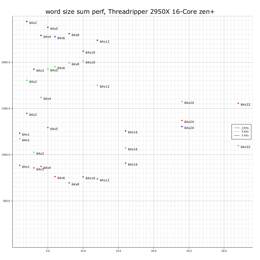
Why is 5-bit precision faster than 4-bit precision for 64x16? Zen+ avx2 has a somewhat unusual architecture, so perhaps we should ignore it.
AWS m6i.32xlarge: Ice Lake (with AVX512 VPOPCNTDQ) 128 vCPUs (64-core, 128-thread)
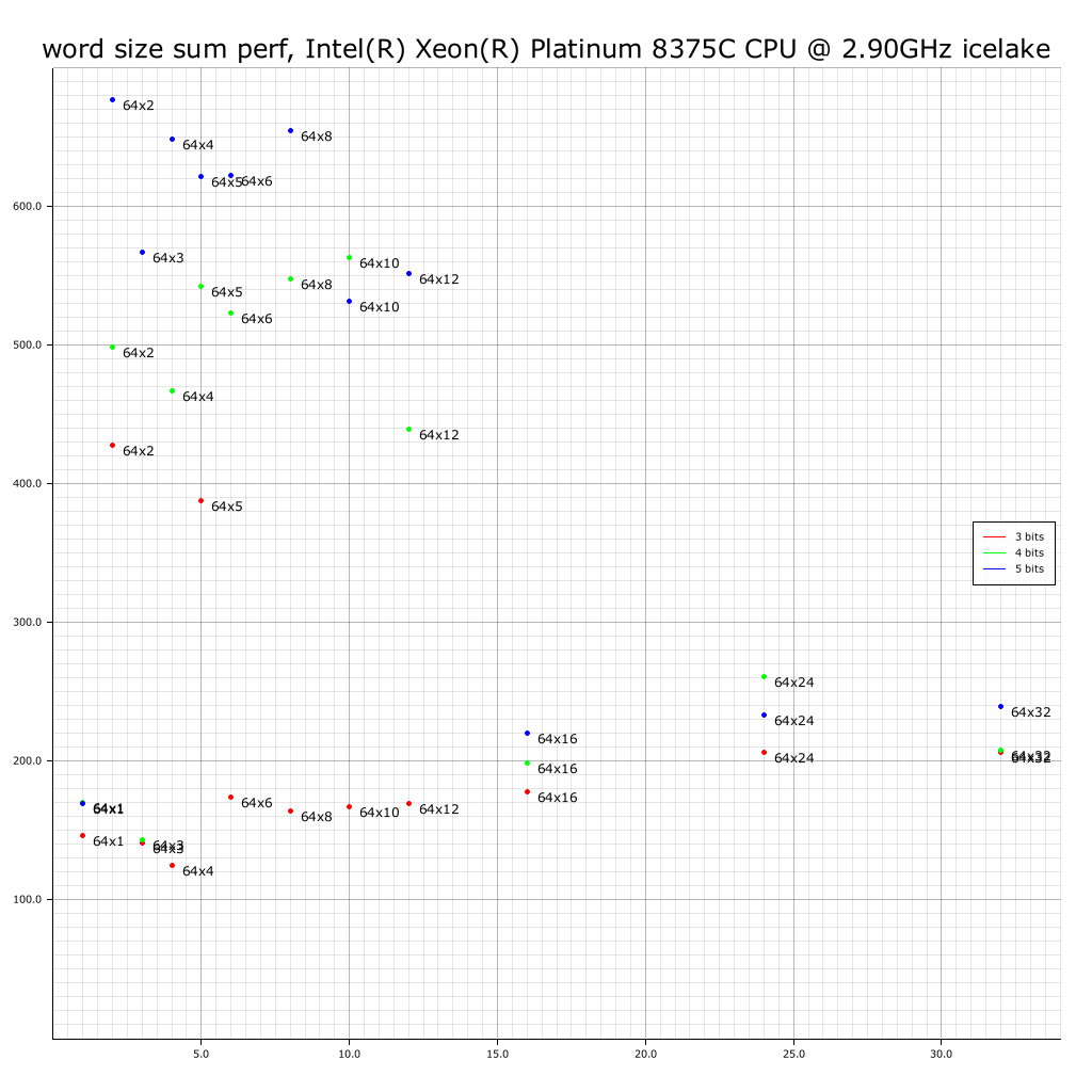
Why is 64x3 such good performance at 4-bit? Why is 64x1 so good at 4 and 5 bits? Is this compiler cleverness or CPU cleverness?
AWS c6g.metal: Graviton2 64-core ARM
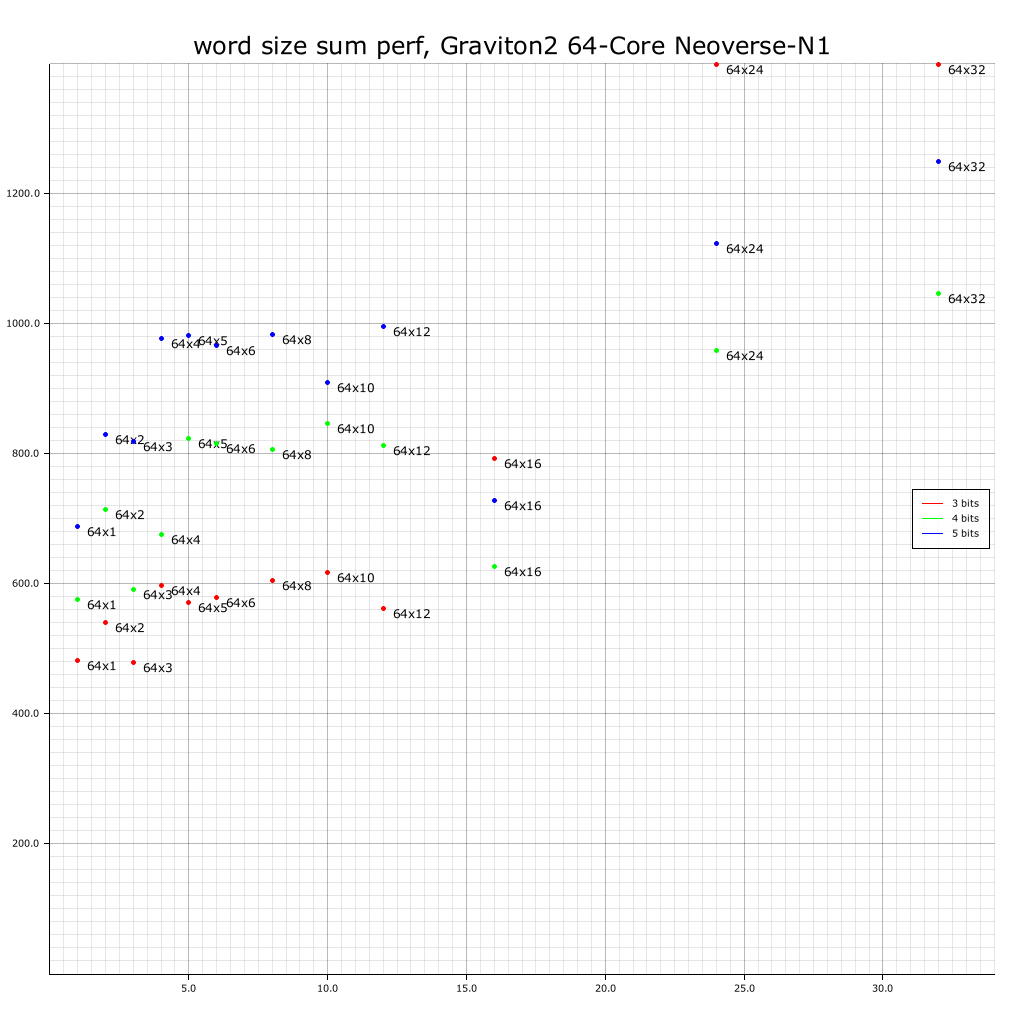
Again, 64x1 at 5 bits is surprisingly good. Why is 64x24 so extremely bad?
The architecture-independent compiler front end is being intermittently clever, and the architecture-specific compiler back end is being intermittently clever, and the CPU/cache is being intermittently clever. Plausibly, this stack of intermittent cleverness explains much of the odd performance behavior.
We invite interested readers to examine the machine code produced for different parameters and attempt to understand it themselves.
Source code
Source code can be found here.
The source code is ~1200 lines of pure, non-unsafe Rust.
The only significant dependency is the rayon crate, used for data parallelism.
The code compiles and runs on x86_64 and aarch64, and contains no architecture-specific code, although as described, best performance requires you to use a word size appropriate to each different machine.
We perform end-to-end tests to demonstrate that for 65536 random examples it produces bit-identical results.
Perhaps someday proof assistants will be sufficiently advanced to permit a formal proof of equivalence.
The code uses the features int_log, adt_const_params, and generic_const_exprs and hence currently requires Rust nightly.
Replicating plots
To run tests:
time cargo run --release --bin count_bits_benchmark -- 25 Tao3 "Genuine Minotaur(R) Xenon(R) Osmium Yarnshredder Baikallake GLORY9 Pineal-A72 Thunderstorm Padua C-WATER Narodnaya-8SV 108-Core @ 7.2GHz" word_perf_tao3.json
Replace 25 with the exponent of the number of examples you want, and other strings as appropriate.
For example, to test on ~2 million examples, use 21.
To generate a plot:
cargo run --bin plot_word_perf -- 3000 word_perf_tao3.json word_perf_tao3.png
To test accuracy on multiple layers:
time cargo run --release --bin layer_demo -- 24 "/path/to/Complete Works of Charles Dickens.txt"
Conclusion
We present a primitive to generate a trit matrix that predicts a target bit-string from an input bit-string, and describe how it can be used in conjunction with the Hadamard matrix to predict bytes.
We utilize bit-slice logic to achieve good performance.
This is cheap to run on distributed commodity CPU cores, requiring only a small number of passes over the training set.
Limitations
Even if these techniques work as expected, they will have many inherent limitations:
- We have no strong evidence that it will actually achieve good accuracy when layers are stacked.
- Even if it can memorize the training set, as a 1D conv net it may well lack the magic token manipulation abilities of transformers.
- This is not a general purpose replacement for end-to-end gradient descent.
- It may only work well on sequence problems where the tokens are ~8 bits in size.
- We see no simple path to 2D conv net training for image classification.
- Training is inherently a batch process; models cannot be progressively trained or fine-tuned end-to-end.
- While potentially cheaper to train than GPT-3, it will still cost several hundred dollars per layer to train on the full The Pile dataset.
Future directions
Multiple layers
We have a primitive that takes two inputs and produces a single target. A single layer gets us to ~34% accuracy. However, we can stack layers. Preliminary evidence suggests that byte-level accuracy grows as we stack layers. However, naive stacking plateaus at ~46%.
It is plausible that skip connections and/or dilation may help. These provide a more powerful node. This node predicts the byte at index i, and takes two inputs. Each input has a negative offset from i, and a pointer to a layer.
Perhaps, we would benefit from more than two inputs. However this would disrupt the chunk and/or word sizes, requiring that we redo cache locality optimizations.
A great benefit of layer-wise training is that we can add layers to the model at will. All existing layers can be reused as inputs to later layers. All layers can act as readout heads, allowing us to easily trade off accuracy against compute cost. Once we have found a node that provides satisfactory performance, we can discard all nodes upon which it does not depend.
Pruning
- All trits that are unset do not depend on their input.
- Activations whose thresholds are outside their activation distribution are fixed.
- Inputs that are fixed need not be computed.
Using these principles, weights may be removed backward and forward. Plausibly, large numbers of weights can be removed while theoretically leaving the model’s behavior unchanged.
This, however, is pointless because a CPU cannot perform sparse inference any faster than dense inference.
E2E pruning
Once a multi-layer model is trained, it is plausible that many of the weights do not provide significant value, or may even be slightly harmful. These weights could be removed with little impact to the model’s behavior.
This, likewise, is pointless because CPUs cannot perform sparse inference any faster then dense inference.
Saving AVX512: Applying an AND Inverter Graph optimizer to the gate DAG and compiling it into VPTERNLOGD bitslice logic for faster inference
In practice, the graph of gates at inference time is sparse; ~98% of the trits are zero. This is difficult to exploit on traditional CPUs. However, just as with training, we can use bitslice logic to compute a sparse DAG of binary operations. However, while compilers are skillful at tasks such as ordering the nodes of a DAG such that the edges can be mapped to a finite set of registers, they are not good at optimizing complex DAGs of boolean logic.
The compiler fails to make optimal use of VPTERNLOG instructions. This is disappointing.
However, the FPGA people have been optimizing DAGs of binary operations and mapping to LUTs for many years. We can potentially use some of their work to map our operations to LUT3s, both for the training code, and, perhaps more importantly, for inference. As long as we can perform inference on 512 examples in parallel, we can have good performance on AVX512 machines.
This will also permit good performance on other machines that lack VPTERNLOGD and have narrower registers, but requires that we build logic out of binary gates rather than LUT3s.
Porting to GPU
It is plausible that the bitslice training implementation could have better price performance on a GPU. A g4ad.xlarge provides an AMD Radeon Pro V520 GPU with 36 Compute Units (CU), and 8GB of HBM2, for only $0.378 per hour. If we (foolishly) attempt to compare a CPU to GPU, a g4ad.xlarge should have ~20x better price performance than a m6i.32xlarge for our use-case. However, GPU programming is painful, and due to the large size of accumulators, one cannot assign each GPU thread a private accumulator. We will need to rethink some of the parallelism. This would be a complex and painful task. Programming GPUs is suffering.
<ignorant_gpu_speculation>
Some thoughts on an implementation:
Consider the case of unit search.
If we perform bit matrix transposition on CPU and send transposed data to GPU, we have a buffer of inputs and target on GPU.
Assume that we compute partial sums on CPU.
Our accumulator is of shape [[[[u32; 2]; 2]; 512]; 256]
A naive approach would be to assign a GPU thread to each of the 256*512*2 = 262,144 counter pairs. This should be sufficient to keep the 64*64*40 = 163,840 threads of a Vega64 busy.
If needed, we could run a few large chunks in parallel, perhaps streaming them from CPU.
Will this be bottlenecked by GPU memory bandwidth?
Since my understanding of GCN is limited, I should probably not attempt to reason about performance, but I will do so anyway.
Each cycle, each compute unit can perform a single binary bitwise operation on all 64 stream processors, for 2048 bits in total.
We do not need to consider accumulator size because each stream processor has its own single private accumulator element which can easily stay in register.
Let us assume that we need to load a word of data every three binary operations.
Given that HBM2 can perform a single 2048-bit transfer per cycle, we can keep up to three compute units fed.
We have made accumulator memory bandwidth negligible, but have vastly increased example data bandwidth requirements.
This is likely not good performance.
Perhaps we could chunk data somewhat.
For example, what if we assign 8x8 chunks of input x target to each stream processor?
Now each stream processor is handling 64 accumulators, and must load 16 words to perform 64*3 cycles of compute.
This should allow 12 CUs to operate.
This still does not fully utilize the CUs of most GPUs.
Perhaps CU local caching will help to reduce RAM bandwidth?
We could go larger; however we are already beginning to have fewer work units than GPU threads.
The PlayStation 4 has a respectable 18 CU GCN GPU, and runs Linux thanks to marcan. Perhaps in a year or two, if used PS4 prices drop, we could do our training on a cluster of PS4s. Given an electricity cost of $0.07 per kWh, we estimate very approximately a factor of 20 times improved price performance compared with AWS GPUs, after initial hardware costs have been amortized.
But at this point, this is all pure speculation. Programming GPUs is suffering.
</ignorant_gpu_speculation>
Acknowledgments
I thank Noah Walton, James Crook, Luke Pflibsen-Jones, and Egan Ford for insightful discussion and helpful suggestions.
All mistakes are my own.
Omake
Daemonic Bean machine
Consider Galton’s bean machine.
In each layer, the falling bean is randomly bopped to one side or the other. Since this is random, the beans will form a normal distribution. As we add more layers, the distribution becomes wider; if we had no layers, the distribution would have no width.
But consider if, instead of a layer being random in the direction to which it bops the bean, the layer has a daemon who is watching the bean and choosing the side to which to bop it. If the daemon has a preference for one side or the other, the distribution will be skewed.
Now suppose that half of our beans are ana while the other half is kata (where kata and ana are two types of beans).
We want the ana beans to be on the left and the kata beans to be on the right.
How do we tell if a given bean is ana or kata?
Some daemons can occasionally recognize certain of the traits correlated with being ana or kata.
We have 512 daemons to work with, but they are not all equally skilled.
Some are better at distinguishing ana from kata, and some are differently good at distinguishing ana from kata.
Different daemons have different failings:
- Some always bop beans to a particular fixed side
- Some are essentially blind and hence bop the beans at random
- Some can distinguishing
katafromanabetter than random but are confused as to which way is right and which way left
Note that the order of daemons is irrelevant; only membership and sign matter.
How are we to select which sets of daemons to use, and by what sign to have each daemon invert its actions?
As we add or remove daemons, or instruct them to flip their direction, the two distributions (of kata and ana) shift independently.
Note that we do not care how far to one side of the center a bean lands.
We win if a kata bean lands left of center, and loose if it lands right of center.
And we can move the center.
Win/loss is boolean; our score is the number of beans that land on the correct side, not how far on the correct side they landed.
If daemons were fully independent, we could choose some threshold of accuracy and reject all daemons below it, but although they are not fully correlated, neither are they fully independent.
How are we to choose which set of daemons to help us sort the beans?
Vehicle selection
Long ago, people rode over the plains in their ox carts; if the axle hole of the cart wheel was well formed, they rode in comfort, and if the axle hole of the wheel was badly formed, they experienced suffering.
Today, as I sit in my room and the fans of my computer spin in their exquisitely machined bearings to move the air to dissipate the heat generated as my Ryzen turns upon the wheel of computation ~4 billion times per second, I experience dukkha because my computer, with all its 16 Zen cores and 128 GB of RAM, takes on average a whole 500 ns to perform 2^18 5-bit integer additions and comparison pairs.
I could practice mindfulness. Perhaps if someone said to me, “Goat carts and deer carts are outside the gate where you can play with them,” I would go outside and play with the goats, and feed them tasty leaves, and scratch their heads, and I and the goats would be free of our respective wheels. But, TFW no goats. :(
Seeing as I have no goat cart to help me, let us consider Johann Tetzel instead.
As the coin in the coffer rings
So the soul from purgatory springs
Perhaps if I gave coin to AMD (who would give some of it to TSMC (who would give some of it to ASML)) to buy a more powerful computer, I could achieve happiness.
But what sort of computer? Should we buy a flock of RPi4s, or a Threadripper 3990X, or perhaps a cluster of PS4s?
To return to wheels, is it better to use the Greater AVX512 Vehicle, the Lesser NEON Vehicle, or perhaps the Lattice Diamond Vehicle? Is it not said that computers are bicycles for the mind? Did not Albert Hofmann ride his bicycle home when he first achieved enlightenment? Surely, vehicles are critical to attaining success, but what sort of vehicle? Is it better to use CPU, or GPU, or FPGA? Is a cluster of RPi4s worth considering? Is a cluster of PS4s worth considering? Which sort of vehicle will better help us to achieve enlightenment most quickly, and, more importantly, most cheaply?
In the summer, my photovoltaic electricity is approximately free, but for others, it is not. In the winter, for people who heat with electricity, electricity is approximately free, because computers are devices for turning electricity into heat which happen to produce computation as a side effect. In order to perform a MapReduce over 825GB of our data in a reasonable time we must use lots of compute in parallel.
Also, our compute demands are spiky. Rather then buy, perhaps we should rent? Whose core GHz hours offer the best price/performance?
This is an easy question to answer with some manual spot market scraping.
| type | spot price | vCPUs | RAM |
|---|---|---|---|
| t3.nano | $0.0016 | 2 | 0.5 |
| t3.micro | $0.0031 | 2 | 1.0 |
| t3.small | $0.0069 | 2 | 2.0 |
| t3a.nano | $0.0023 | 2 | 0.5 |
| t3a.micro | $0.0030 | 2 | 1.0 |
| t3a.small | $0.0063 | 2 | 2.0 |
| t2.micro | $0.0035 | 1 | 1.0 |
| t2.small | $0.0069 | 2 | 1 |
| a1.medium | $0.0084 | 1 | 2 |
| m6g.medium | $0.0179 | 1 | 2 |
| c5.large | $0.0335 | 2 | 4 |
| c4.large | $0.0312 | 2 | 3.75 |
| GCP n1-standard-1 | $0.01 | 1 | 3.75GB |
| GCP n1-highcpu-2 | $0.014 | 2 | 1.80GB |
| IBM classic transient | $0.019 | 2 | 4 |
| Azure A1 | $0.012 | 1 | 1.75 |
| Azure A1 v2 | $0.009 | 1 | 2 |
| Azure D2a v4 | $0.022 | 2 | 8 |
| Azure D1 | $0.015 | 1 | 3.5 |
| Azure F1 | $0.012 | 1 | 2 |
| Azure A0 | $0.018 | 1 | 0.75 |
Some spot instances are cheaper then others per core.
But they also vary in terms of performance.
What merit do we gain by paying half the price per hour if it must run three times longer?
Some have AVX512, others do not.
The x86 cores are merely hyper threads, not physical cores.
Will our co-tenants share L1/L2 cache nicely?
The t* types are cheaper, but they are also shared-core.
a1 and m6g are ARM based.
Do we care?
Consider a developer who needed to provision a VM, who said: “I will not use the VM until I know whether it was designed by an Israeli, Korean or an American’ He would say, ‘I will not use the CPU until I know whether it was laid out by a human or by a neural net… until I know what feature size, and how many layers… until I know whether the motherboard was made by Dell, SuperMicro, HP, or Lenovo… until I know whether it is using KVM or Xen.” The developer would be fired and those things would still remain unknown to them.
Next: Porting to GPU and large scale benchmarking of small spot machines on public cloud